2018 ICPC World Finals

May 2, 2018, 12:40 pm

The ICPC World Finals in Beijing just wrapped up, and I had the great privilege of representing the University of Texas with my teammates, Arnav Sastry and Daniel Talamas. This was the first time any of us competed at the World Finals, and it was an amazing experience.

My team didn't perform as well as we'd hoped, but we didn't do embarrassingly poorly either. We ended up solving four problems (out of eleven) and placing 65th (of 140). Here, I'll write a brief summary of our experience in the competition.

Getting started

When the countdown finished, Arnav logged into the computer and handed me the problem packet. While Arnav was writing our .vimrc, .bashrc, and template, I started reading the problems front-to-back while Daniel read back-to-front. I told Arnav that B looked like an implementation problem, and, being the fastest typist on our team, he took a look and started coding.

While Daniel and I continued reading problems, other teams got accepted verdicts on three problems: F, B, and K. I diverted my attention to K.

First AC

While Arnav coded B, I came up with a greedy constructive algorithm for K. Soon I convinced myself of its correctness, and as soon as Arnav submitted B I took the keyboard to code K. Arnav's solution to B got accepted, and we celebrated our quick AC. The solution to K was relatively simple to implement, and it was finished in just a few minutes. Passing samples, I asked Daniel for a sanity check on my idea and submitted K.

Seventh place

Arnav got back in the hot seat and began coding a solution to G using Java's AWT library. Geometry has historically been our weak point, but we know how to do basic things like polygon union and intersection using this library. In the past we have gotten some tricky geometry problems with this trick, so with nothing else to code we decided it was worth a shot. We didn't have high hopes, because at this point no other team had gotten G.

In the meantime, our K solution got accepted, and we rose to 7th place on the leaderboard.

Arnav finished our solution to G, and running on samples it was nowhere near accurate enough. The sample output was 50, and our code gave 49.997. With no ideas for a real solution, we gave up on G for the time being.

DP on edges

At this point, Daniel figured out the solution to A: a DP on edges. He explained it to me, and I started to code, but he preempted me and coded it himself. Unfortuately, the code failed samples, and it took us a very long time to find the bug: in our DFS, we forgot to update the memoization table.

While Daniel tried to find his bug, Arnav worked on F (the apparent next easiest problem) and I worked on C. I mistakenly thought that some team had already gotten AC on C, and I had an idea that I thought could work. As I wrote pseudocode, it became clear that my idea had a big flaw, and Daniel pointed out that no one else had C, so I abandoned it.

Arnav was unsure if his solution to F would run in time. He coded it anyway, and it gave wrong answer. Daniel found his bug in A and submitted, getting accepted.

Time limit squeezing

We knew that if we could get F, H and I were our next best bets. Unfortunately, even after finding an edge case and fixing a bug in F, we got TLE. After some more optimizations, we got another TLE; after one more, WA. Finally, we fixed that bug and got AC, but with a massive penalty for wrong submissions. We found out after the contest that some teams wrote a solution without the optimizations we included, but broke early when nearing the time limit, and these solutions got AC as well. I'm very impressed by the teams that got F on their first attempt!

H is for hard

H was another geometry problem: find the minimum number of line segments you need to use to cut every wire going across a rectangular door (also given as line segments). Arnav and I realized quickly that you can always do it in two cuts, so all that is needed is to check if it is possible in one. Thinking what remained would be easy, we focused our attention on H rather than I, the other problem that may have been within reach.

This turned out to be a mistake. We spent the last two hours trying to get H, with only a few wrong attempts and wrong conjectures. In hindsight, our strengths were much more in favor of I. Nonetheless, while Arnav and I coded H, Daniel thought about I.

The hard part of H (like many geometry problems) is finding the right WLOGs: there were up to \(10^6\) line segments, so the obvious \(O(N^2)\) sweep line approach doesn't work. We needed some way to reduce the runtime.

We guessed that our cut should always link two opposing sides, and we tried an approach that produced four candidate line segments and then checked all of them. Although it passed every case we could think of, it gave WA when we submitted.

The worst part: we still don't know how to solve it. We figured out I on the plane ride back to the States, but H still eludes us. I fear that I will be haunted by this problem forever.

Wrapping up

We spent the last 10 minutes speed-coding a solution for H based on another (incorrect) conjecture, but we couldn't finish in time and so we didn't get to submit it.

We were disappointed to have only solved four problems, but we had a great time at the contest. The problems were generally interesting, and I hope to return next year, wherever it ends up being!

K revisited

My favorite problem of the set was K (probably because I solved it). You are given a graph with \(N\) vertices and \(M\) edges, and you want to construct a tree with \(N\) vertices that minimizes the number of nodes whose degrees differ from their respective degrees in the original graph.

The obvious greedy thing to do is write down the degrees of each node, and, while the sum of the degrees is greater than \(2N - 2\), cut the largest degree down to \(1\) (or to some other value if changing it to \(1\) would remove too many edges).

The question is: given our new degree sequence, can we construct a tree with these degrees?

My approach was to sort the nodes again by their new degrees, and build a rooted tree. We keep a stack of nodes who don't have parents, and for a node \(u\) with degree \(d\) we pop \(d - 1\) nodes from the stack and assign them parent \(u\). We must special case the root.

It was not immediately obvious that this process never gets stuck (tries to pop from an empty stack). While Arnav coded B, I came up with a nifty proof. Let \(D\) be the degree sequence. If we are trying to add node \(k + 1\), the number of nodes currently in our active stack is \(k - \sum_{i=1}^{k} (D[i] - 1)\). Simplifying, this is \(2k - \sum_{i=1}^{k} D[i]\).

We want to show that this is always at least \(D[k + 1] - 1\). Rearranging, we want

\[\sum_{i=1}^{k+1} D[i] \leq 2k + 1\]

for all \(k\).

We can't prove this using standard induction, because when we are partway through the process we don't know anything about the future degrees. In fact, the only restriction on the future degrees is that the sum of all degrees is \(2N - 2\).

But then the claim is obvious for \(k = N - 1\): \(\sum_{i=1}^{N} D[i] = 2N - 2 \leq 2N - 1\). The off-by-one here is because we want a slightly stronger claim for the last node (because the root does not get a parent). But we satisfy this stronger claim too.

For \(k = 0\), the claim is obvious as well: the first degree must be \(1\), since the degrees are sorted and if all degrees are at least \(2\) the sum of degrees must be at least \(2N > 2N - 2\).

So the partial sum of degrees is under the linear function at the beginning and at the end. How can we show that it is under the linear function along its entire domain?

Since we ordered the degrees in increasing order, the partial sum of degrees as a function of \(k\) is convex! A convex function always stays under the line connecting two points on its graph. This completes the proof that the construction works for any degree sequence with the right sum, including the greedy sequence we found earlier.

The other problems of the set were also interesting, but this was the one from which I learned the most.

It's been a while since I posted on this blog, so hopefully I start doing that more in the coming months. I probably won't, but I will try. Thank you for reading!

Trees on Graphs

April 4, 2017, 11:02 pm

A couple of weeks ago, I was solving a Codeforces problem and I came across a trick I hadn't seen before. Here, I'll give that problem, describe the solution, and then show how to apply it to a more complicated problem.

Codeforces 786B: Legacy

In this problem, we are asked to compute the single source shortest paths in a weighted directed graph, with all the weights nonnegative. The catch: there are three types of edges. There are normal edges of the form \((u, v)\), but there are also edges that look like \((u, [l, r])\) and \(([l, r], u)\). Here, \([l, r]\) refers to all the nodes whose index is between \(l\) and \(r\), inclusive. There are up to \(10^5\) nodes and edges.

The naive solution is to convert all edges of the form \((u, [l, r])\) to \(r - l + 1\) edges of the form \((u, i)\) (and to do the same for all edges of the form \(([l, r], u)\)). Of course, there are \(O(N \cdot M)\) edges in this transformed graph (where \(N\) deontes the number of nodes in the original graph, and \(M\) is the number of edges), so this solution will MLE or TLE.

Let's digress for a minute and consider a different problem: given an array of numbers and \(Q\) queries, each of the form \([l, r]\), output the minimum value in the subarray defined by each query. There are multiple solutions to this problem, but perhaps the most common is to use a segment tree: we build a binary tree on top of the array and decompose queries into \(O(\log N)\) disjoint intervals (represented by nodes in the tree) whose union is the desired query.

For example, say the array is \([5, 3, 5, 10, 7, 2, 8, 14]\), and our query is \([3, 6]\) (we are using \(1\)-indexing). This query can be represented as the union of \([3, 4]\) and \([5, 6]\), two nodes present in our segment tree.

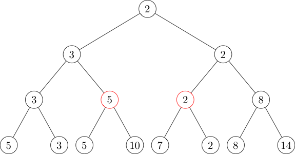
The two red nodes represent the intervals \([3, 4]\) and \([5, 6]\), so if we identify them in \(O(\log N)\) time we can then find the answer to our original query in \(O(\log N)\) time by taking the minimum of the values in those nodes. (Exercise: prove that all intervals are the disjoint union of \(O(\log N)\) nodes, and code a segment tree.)

Now, back to our shortest paths problem. We will use the same idea: decompose an interval \([l, r]\) into \(O(\log N)\) disjoint smaller intervals on which we can do some preprocessing.

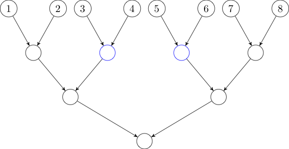
In this case, we will need two trees: one with edges directed down the tree and one with edges directed up the tree. All these edges will have weight zero.

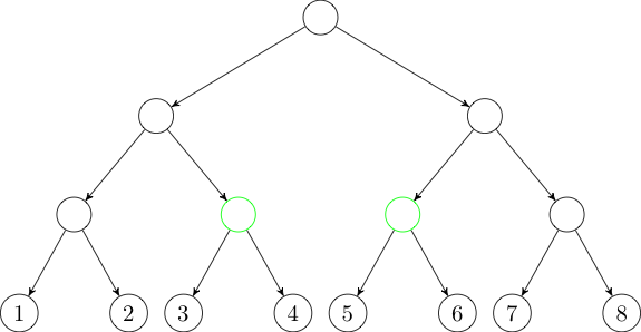
Now, if we want to add an edge from some node to the interval \([3, 6]\), we can instead add an edge to each of the two green nodes in the first tree. Similarly, if we want to add an edge from the interval \([3, 6]\), we can instead add an edge from each of the two blue nodes in the second tree.

We've added \(O(M \log N)\) edges to our graph, and running Dijkstra's algorithm on the new graph easily runs in time.

AtCoder RC069F: Flags

This problem is from a recent AtCoder contest. I didn't get to do this contest live, but I found the problems really enjoyable. Flags was the hardest problem, largely because it combines a few different techniques.

We want to place \(N\) flags in a line while maximizing the distance between the closest two flags. Each flag has two positions in which it is allowed to be placed, and \(N\) can be up to \(10^4\).

We will binary search on the answer; denote our current guess \(d\). Checking whether it is possible to place all the flags with at least distance \(d\) between every pair is a 2-SAT problem.

A common technique for solving a 2-SAT problem like this is to build the "implication graph": a directed graph in which the nodes represent boolean variables and their negations, and edges represent logical conditionals. So an edge exists between two nodes \(u\) and \(v\) if \(u\) "implies" \(v\), and if we assign \(u\) the truth value "true", then \(v\) must also be marked "true". Then the 2-SAT problem is satisfiable if it is not the case that some node directly or indirectly implies its negation, and its negation directly or indirectly implies the node itself. We can easily check this condition by finding the strongly connected components of the implication graph.

So let's build the implication graph. Each flag has two nodes, one for each of its possible locations. We will assign each of these nodes a truth value, and we require that, for a solution to be valid, the two nodes associated with each must be assigned opposite truth values. That is, each flag must be placed in exactly one of its two positions. For convenience, we will say that if node \(u\) represents placing a particular flag in its first location, then \(\neg u\) refers to the node representing placing that flag in its second location (and vice versa).

We will add an edge from \(u\) to \(\neg v\) if the distance between the posistions associated with \(u\) and \(v\) is less than \(d\). This edge indicates that if we assign \(u\) "true", then all the potential positions that are nearby are disqualified: for all of those flags, we must take the other option. Implementing this naively will yield a time complexity of \(O(N^2 \log X)\), where \(X\) is the size of the space over which we're binary searching (probably \([0, 10^9]\)). This is too slow.

However, if we sort all our nodes by position (breaking ties arbitrarily), then we can binary search before and after each node \(u\) to get two intervals of nodes. We want to add an edge from \(u\) to the negation of every node in those intervals.

That we're adding edges to intervals is a big hint to use the tree-on-graph technique we used in the previous problem. If we can use that trick here, we will reduce our number of edges from \(O(N^2)\) to \(O(N \log N)\). And in fact, the trick works the same way here, with an extra hiccup. Our tree's leaves shouldn't connect directly to the nodes they represent, but rather to their negations. The implementation is still straightforward, but this shows that we can use the tree-on-graph trick even when the ordering of nodes we use to build the tree is different than the ordering we use to decide what intervals to query when we add additional edges.

Consider the following sample case.

4
1 3
2 5
1 9
3 8

There are four flags. The first one can be placed at position \(1\) or \(3\), the second can be placed at \(2\) or \(5\), the third can be placed at \(1\) or \(9\), and the fourth can be placed at \(3\) or \(8\).

First, we will create our 2-SAT nodes. \(s\) will be the node representing placing the first flag at position \(1\), and \(\neg s\) will be placing the first flag at position \(3\). The same pattern will be used for \(t\), \(\neg t\), \(u\), \(\neg u\), \(v\), and \(\neg v\).

Below are the nodes in their natural order.

Next, we will build our tree so that we can add edges to intervals. Note that the leaves of the tree are the negations of the nodes in the natural order above.

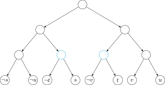
Now, if we want to add an edge to the negations of the node in the interval \([3, 6]\), we can just add an edge to each of the nodes marked in cyan.

This completes the solution to the problem. There are \(O(N \log N)\) edges in our new graph, and we can build the implication graph, find its strongly connected components, and ensure that no node is in the same SCC as its negation.

In this problem, the "trees on graphs" technique was only a small part of the whole solution, but for me it was the hardest part to see. In general, this technique can be used whenever we have a graph where some edges are to or from intervals of the nodes (under some ordering). The only caveat is that we must ensure that we preserve the properties of the graph we need for our solution. In the first problem, we needed to preserve path costs so that Dijkstra's algorithm would work. In the second problem, we needed to preserve the implication relationships between nodes: if (and only if) node \(u\) is reachable from node \(v\) in the original graph, \(u\) should be reachable from \(v\) in the transformed graph.

Keeping that in mind, I'm sure this can be applied to many other problems. I look forward to solving more of them in the future!

Codeforces Educational Round 18

March 29, 2017, 7:28 am

I haven't participated in many Codeforces rounds lately, but I did do Educational Round 18. Codeforces hosts "Educational Rounds" periodically, which are unrated and usually focus on teaching common techniques and tricks.

Problem C was a simple greedy algorithm with lots of edge cases, and problem D was essentially implementation. Problem E was interesting, but unfortunately I couldn't solve it during the contest. Nonetheless, here are my thoughts on it.

E: Colored Balls

In this problem, we have \(N \leq 500\) colors of balls (with \(x_i \leq 10^9\) balls of color \(i\)), and we want to partition the balls into monochromatic sets such that no two sets differ in size by more than \(1\). Our goal is to minimize the number of sets.

First, it is clear that this is the same as maximizing the number \(k\) such that every set is of size \(k\) or \(k + 1\): after finding this number, we can find the minimum number of sets for a particular color \(i\) by taking \(\lfloor \frac{x_i}{k + 1} \rfloor\) and then adding \(1\) if the remainder is nonzero. (To see why, consider a variant of the division algorithm: \(x_i = q(k + 1) - r\), with \(0 \leq r \leq k\). The above procedure gives us \(q\) in this formulation, and that corresponds to taking \(q - r\) sets of size \(k + 1\) and \(r\) sets of size \(k\).)

Each \(x_i\) has some number of potential valid values of \(k\), and we want to find the maximum \(k\) that is valid for all \(x_i\). Our approach will be as follows: generate the whole set of valid \(k\) values for \(x_1\), and then cull this set for each of \(x_2, x_3, \dots\).

There are a few parts to this solution. First, let's try to characterize the valid values of \(k\) for a particular \(x_i\). We want to know for which values of \(k\) there exist nonnegative integers \(a, b\) such that \(x_i = a(k) + b(k + 1)\). Since \(k\) and \(k + 1\) are always coprime, there are infinitely many (potentially negative) integers \(a\) and \(b\) satisfying this equation. If we can find one solution, then we can characterize all the solutions. The obvious solution is to take \(a = -x_i\) and \(b = x_i\), so all the solutions are of the form \(a = -x_i + (k + 1)z\) and \(b = x_i - kz\), for \(z \in \mathbb{Z}\). If there are any solutions with both \(a \geq 0\) and \(b \geq 0\), then one such solution will be with \(z = \lfloor \frac{x_i}{k} \rfloor\). \(b\) will always be nonnegative with this value of \(z\), so we only need to check if \(a \geq 0\) also: \(a = -x_i + (k + 1)\lfloor \frac{x_i}{k} \rfloor \geq 0\), which is the case when \(\lfloor \frac{x_i}{k} \rfloor \geq x_i \bmod k\) (where \(\bmod\) is taken to mean remainder, as in most programming languages).

This gives an easy way to check if a given value of \(k\) will work for a particular \(x_i\), and so we can use this in the culling step in our algorithm. However, this doesn't help us generate all the valid values for \(x_1\). It's not even clear that there aren't too many values to store in a set!

It turns out that there are never more than \(3\sqrt{x_i}\) values of \(k\) for any \(x_i\). To prove this, we will just describe the procedure to enumerate them; this will also complete our algorithm.

First, note that for \(k \leq \sqrt{x_i}\), the condition (\(\lfloor \frac{x_i}{k} \rfloor \geq x_i \bmod k\)) always holds. This gives us \(\sqrt{x_i}\) values. For the others, we iterate over all possible values of the left-hand side of the inequality (there are only \(\sqrt{x_i}\) to consider), and for each, we identify at most \(2\) values of \(k\) that are valid.

We will denote our guess for the left-hand side of the inequality by \(y\). We will show that only \(\lfloor \frac{x_i}{y} \rfloor\) and \(\lfloor \frac{x_i}{y} \rfloor - 1\) may be valid values of \(k\). It will be easy to check each of these using our condition and add them to our set if they are indeed valid.

So we want to show that only \(k = \lfloor \frac{x_i}{y} \rfloor\) and \(k = \lfloor \frac{x_i}{y} \rfloor - 1\) may satisfy both \(\lfloor \frac{x_i}{k} \rfloor = y\) and \(x_i \bmod k \leq y\). We will show at least one condition must fail whenever \(k > \lfloor \frac{x_i}{y} \rfloor\) or \(k < \lfloor \frac{x_i}{y} \rfloor - 1\).

First, we handle the \(k > \lfloor \frac{x_i}{y} \rfloor\) case. In this case, the first condition (\(\lfloor \frac{x_i}{k} \rfloor = y\)) cannot hold; in fact, \(\lfloor \frac{x_i}{k} \rfloor < y\). It is enough to note that \(k > \frac{x_i}{y}\) whenever \(k > \lfloor \frac{x_i}{y} \rfloor\), since \(k\) is an integer. Then

\[\left\lfloor \frac{x_i}{k} \right\rfloor \leq \frac{x_i}{k} < \frac{x_i}{x_i/y} = y.\]

The \(k < \lfloor \frac{x_i}{y} \rfloor - 1 \) case is more subtle. Without loss of generality, assume the first condition holds (if not, then we are done). We will prove that \(x_i \bmod k > y\). To do so, we again invoke the division algorithm. For convenience, let \(m = \lfloor \frac{x_i}{y} \rfloor - k\).

\begin{align} x_i &= qk + r & (0 \leq r < k) \\ &= yk + r \\ &= y\left(\left\lfloor \frac{x_i}{y} \right\rfloor - m\right) + r \end{align}

But since \(y \lfloor \frac{x_i}{y} \rfloor \leq x_i\), rearranging gives \(r \geq my > y\), as desired.

This completes the proof that there are never more than \(3\sqrt{x_i}\) (in practice, there are usually close to \(2\sqrt{x_i}\)) valid values of \(k\), and so we can start by testing all of these for \(x_1\), adding valid ones to a set, and then iterating over the other \(x_i\) and removing invalid ones. At the end, we can choose the largest element of our set (the set can never be empty because \(k = 1\) is always valid) and calculate the corresponding minimum number of sets as described above.

Codeforces Round #400

February 26, 2017, 6:40 am

Thursday morning, Codeforces hosted the ICM Technex 2017 round. Unfortunately, I wasn't able to compete, but I thought two of the problems were interesting.

D: The Doors Problem

This was a nice 2-SAT style problem. We have a set of \(M\) doors, each of which is locked or unlocked. We also have \(N\) switches (toggling a switch toggles the state of all doors connected to that switch). Furthermore, each door is connected to exactly two switches. We want to know if it is possible to unlock all the doors by toggling some subset of the switches.

So we create a graph with \(2N\) nodes and \(2M\) edges. Each switch \(i\) is associated with two nodes: one of these represents toggling switch \(i\) (denoted by \(u_i\)) and the other represents not toggling switch \(i\) (denoted by \(v_i\)). Each door is represented by two edges. If the door is initially unlocked, then we must either toggle both its switches, or toggle neither. Thus, if the door is connected to switches \(i\) and \(j\), we add undirected edges \((u_i, u_j)\) and \((v_i, v_j)\). On the other hand, if the door is initially locked, we must toggle one of its switches but not the other, so we add edges \((u_i, v_j)\) and \((v_i, u_j)\). Now the nodes of our graph are partitioned into connected components that must be assigned the same truth value: if a node \(u_i\) belongs to a component assigned "true", then we must toggle switch \(i\); if \(u_i\) belongs to a component assigned "false", then we must not toggle switch \(i\). Similarly, if \(v_i\) belongs to a "true" component, then we must not toggle switch \(i\); if \(v_i\) belongs to a "false" component, then we must toggle switch \(i\).

All that remains is to determine whether there is a truth assignment for our components that is consistent: that is, there does not exist an \(i\) with \(u_i\) and \(v_i\) receiving the same truth value. This is the case exactly when, for all \(i\), \(u_i\) and \(v_i\) belong to different components.

This can be implemented by explicitly building the graph and finding the connected components, or by using a union-find data structure.

E: The Holmes Children

In this problem, we are asked to evaluate a function \(F_k(n)\), where \(F_k\) is defined as a composition of \(k + 1\) functions, alternating between \(f\) and \(g\). \(f(n)\) is defined to be the number of ordered coprime pairs \((x, y)\) where \(x + y = n\), and \(g(n)\) is the summatory function of this function: \(g(n) = \sum_{d|n} f(d)\).

First, it is not hard to see that \(f\) is Euler's \(\phi\)-function: \(f(n)\) is the number of positive integers at most \(n\) that are coprime to \(n\). This is because \(\gcd(x, y) = \gcd(x, x + y) = \gcd(x, n)\), and after fixing \(x\), \(y\) is already determined.

Now, it turns out that \(g\) is actually the identity function (\(g(n) = n\) for all positive integers \(n\)). To prove this, recall that \(f\) is multiplicative: that is, for coprime positive integers \(a\) and \(b\), \(f(ab) = f(a)f(b)\), and that the summatory function of a multiplicative function is also multiplicative. Thus, \(g\) is multiplicative, and it will suffice to show that \(g(p^k) = p^k\) for primes \(p\) and nonnegative integers \(k\). To do this, note that the divisors of \(p^k\) are \(1, p, p^2, \dots, p^k\), and that \(f(p^i) = p^i - p^{i-1}\). Then \(g(p^k) = 1 + \sum_{i=1}^{k} p^{i} - p^{i-1} = p^k\) (this is a telescoping sum). Since \(g(p^k) = p^k\) and \(g\) is multiplicative, \(g(n) = n\) for all positive integers \(n\). (This is because we can decompose any \(n\) into prime powers, all of which are clearly coprime.)

So all that's left is applying \(f\) to \(n\) \(10^{12}\) times. First, to apply \(f\) once, we just have to find the prime factorization of \(n\) (recall that \(f\) is multiplicative); this takes \(O(\sqrt{n})\) time. Since \(n\) can be up to \(10^{12}\), it seems as if we have to do \(10^{18}\) operations.

However, repeated application of \(f\) decreases \(n\) very rapidly. To formalize this, we make two observations: first, if \(n\) is even, then \(f(n) \leq n/2\). This follows from the fact that if \(n\) is even, every even integer up to \(n\) is not coprime with \(n\). Second, if \(n \geq 3\), \(f(n)\) is even. This is not too hard to prove: \(f(p^k) = p^k - p^{k-1}\), which is even if \(k \geq 2\) or \(p\) is odd. Since \(f\) is multiplicative, if \(n\) is not \(1\) or \(2\), then \(f(n)\) is even.

So if \(n\) is initially odd, a single application of \(f\) will make it even. Then we need only \(O(\log n)\) iterations to reduce \(n\) to \(1\). Thus, even though the given bound for \(k\) is \(10^{12}\), the answer won't change for \(k \geq 40\) or so, and we can stop early if \(n\) ever becomes \(1\), so our solution will easily run in time.

HackerRank University CodeSprint 2

February 20, 2017, 11:32 am

I realized that I haven't posted anything here since 2014, and it looks bad to have a "blog" with nothing on it. I really enjoyed the problems in HackerRank's University CodeSprint 2 this weekend, so I figured I would write down the ideas from my solutions here.

Problems A (Breaking the Records) and B (Separate the Numbers) were straightforward implementation, and C (Game of Two Stacks) was a basic binary search/two pointers problem. Below are my thoughts on the other three problems I solved.

D: The Story of a Tree

We are given an (undirected, unrooted) tree and a set of queries which are each in the form of a directed edge. We are asked to consider rooting the tree at each of its \(N\) vertices, and in each case to count the number of queries that are "correct"--that is, queries \((u, v)\) in which \(u\) is the parent of \(v\). (It is guaranteed that there is an edge between \(u\) and \(v\).)

The obvious solution is \(O(N^2)\): for every root, DFS on the tree and count the number of correct queries. This will be too slow for this problem, but it's not hard to bring it down to \(O(N)\).

First, we will run the naive solution for an arbitrary root. Then note that the number of correct queries after rooting the tree at an adjacent node can differ by at most \(1\): if the edge we traverse is a query. So we will run another DFS starting at the same node as before (because we know the answer for this root), and every time we traverse an edge, we check if that edge is a query (in each direction, \((u, v)\) and \((v, u)\)) and update our current answer accordingly. Each of the two DFSs is linear, so the solution as a whole is linear.

E: Sherlock's Array Merging Algorithm

We are given the output of a strange array-merging procedure, and we are asked the number of distinct inputs that could have produced this output. The procedure is as follows: we start with a collection of arrays \(V\), and for each iteration, we remove the first item from each array, and insert these \(|V|\) items into our final array in sorted order. Not all the starting arrays have to be the same length (we just remove empty arrays after we remove their last item).

The first observation to make is that each iteration of the merging procedure produces a sorted subarray in the final array. We then want to count the number of ways to partition the final array into sorted subarrays of non-increasing length... sort of. If we do that, we will be undercounting: some partitions correspond to more than one initial collection. For example, partitioning \(123\) into \(12|3\) corresponds to both \(V = [13, 2]\) and \(V = [1, 23]\). Instead of saying \(DP[i][j]\) is the number of ways to partition the first \(i\) elements with the last partition having size \(j\), we will call it the number of "permuted partitions". (I'm not sure if there is a formal name for this.) Intuitively, we want to multiply by the number of ways to match up this segment with the previous one.

Then it is clear that \(DP[i][j] = \sum_{k \geq j} (DP[i-j][k] \frac{k!}{(k-j)!})\). These transitions are \(O(N)\), and there are \(O(N^2)\) states. With constraints of \(N \leq 1200\), I expected this to time out, but as it turns out, because of the small constant factor this is fast enough. I suspect there is a way to reduce the time to \(O(N^2)\), but I'm not sure how.

G: Minimum MST Graph

This problem took me all day Saturday, largely because I had an off-by-one bug in one of my for loops but I was sure the error was elsewhere.

We are given \(N\), \(M\), and \(S\)--the number of nodes, number of edges, and MST weight--of an unknown graph. Our goal is to give the minimum sum of weights of edges in a graph satisfying these three criteria.

First, instead of giving each edge a weight, we will give each node a weight. Each edge's weight is then the maximum of the weights of its two endpoints. We will assume that node \(0\) has the smallest weight, node \(1\) has the second smallest, etc., and furthermore that node \(0\) has weight \(0\) (every other node will have weight at least \(1\)). We will define an array \(B\) based on these values. That is, \(B[i]\) is the weight of node \(i\).

Now we will define a second array \(A\) which contains information about the structure of the graph we are constructing. In particular, \(A[i]\) is the number of "backward edges" from node \(i\). If an edge connects nodes \(i\) and \(j\) where \(i < j\), we say that edge is a "backward edge" from node \(j\). This is useful because of the ordering of the nodes: the weight of node \(i\) is no more than the weight of node \(j\), and so the weight of an edge is the same as the weight of the node for which it is a backward edge.

So we have \(B[0] = 0\), and \(B[i] \geq 1\) for \(i > 0\). We also have \(A[0] = 0\), and \(1 \leq A[i] \leq i\) for \(i > 0\). (If \(A[i] = 0\), then our graph may not be connected, and even if it is, we can make our answer no worse by making all \(A[i] \geq 1\); if \(A[i] > i\), then it must have multiple edges or self loops. I encourage you to verify this for yourself.) For simplicity, we will stop considering node \(0\) from now on, and assume that our arrays are only defined on indices \(1 \leq i \leq N - 1\).

Note that \(\sum A[i] = M\) and \(\sum B[i] = S\). Subject to all these constraints, we want to minimize \(\sum A[i] B[i]\).

This is a much more manageable and comprehensible problem, but it still seems hard. First, let's suppose \(B\) is fixed and build an optimal \(A\). To do this, first recall that \(B\) is increasing (albeit not strictly). Now, we can set \(A[i] = 1\) for \(1 \leq i \leq N - 1\). We will add the remaining \(M - (N - 1)\) edges to our graph greedily. For each edge, we should increment \(A[i]\) for the smallest \(i\) that is not yet "full"--that is, for which \(A[i] < i\). It is easy to see that this will lead to an array \(A\) with some prefix of its elements being set to their index, potentially followed by at most one element that is not \(1\), potentially followed by a bunch of \(1\)s. So it turns out that \(A\) does not depend on \(B\) at all; that is, the structure of our optimal graph depends only on \(N\) and \(M\)!

Having found \(A\), we only have to find the array \(B\) that minimizes \(A \cdot B\). There is a greedy algorithm for this, too: let \(C[i]\) be the "cost" of incrementing the last \(i\) elements of \(B\). It is equal to the sum of the last \(i\) elements of \(A\), divided by \(i\). Intuitively, \(C[i]\) is the amount by which our answer increases per unit of weight we allocate. Then if we currently have \(X\) weight to distribute, we find the \(i \leq X\) for which \(C[i]\) is minimum, and we increment the last \(i\) elements of \(B\). When we have no more weight to distribute, we are done. Simply computing the desired dot product yields the answer.

With reasonable implementation, this algorithm has time complexity \(O(N + S)\), which will pass all but the last subtask (getting 70% score). The last subtask isn't as interesting: it just takes some careful reasoning and algebra to find a closed-form answer that can be computed in \(O(1)\) time.

Well, thanks for reading, and maybe I'll post some more competitive programming-related stuff on here in the future if I again find myself trying to avoid doing homework.

Hello, World!

November 23, 2014, 2:09 pm

I've created this website to serve as a personal portfolio and résumé. I hope to post occasional updates about my life or technical things on this blog.

If you want to hire me or chat, please email me at ethan @ this website.

Thanks!